Hydraulic Model Cheat Sheet
⏯
❮

 ❯
❯
1 / 15
2 / 15
3 / 15
4 / 15
5 / 15
6 / 15
7 / 15
8 / 15
9 / 15
10 / 15
11 / 15
12 / 15
13 / 15
14 / 15
15 / 15
Variables
There are a few important variables and equations to know in order to understand how groups move within the Hydraulic Model.
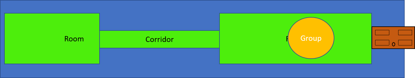
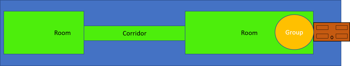
Group variables
These can change as the group moves:
- Density: $D \; [ppl/m^2]$
- Speed: $S \;[m/s]$
- Specific flow rate: $f\; [ppl/s/m]$
- Calculated flow rate: $F\; [ppl/s]$
Element-specific variables
These remain constant for that element:
- Density-Speed coefficient: $k_{i} \; [m/s]$
- Effective width: $W_{eff,\;i} \;[m]$
Global constant
This remains constant for all elements and groups:
- $a\; [m^2/ppl]$
Equations
To find the speed ($S_i$) of a group within an element, we must know which element they are in, and their local density: $$𝑆_{i} = (1−𝑎𝐷_{i})𝑘_{i}$$
Once we know the speed of a group, we can also determine the flow rate within that element, using the effective width ($W_{eff}$), and the specific flow rate ($f$): $$F_{i}=f_{i}W_{eff, \; i}$$ The specific flow rate is calculated by: $$f_{i}=S_{i}D_{i}$$ Which then yields the actual flow rate: $$ F_{i}=S_{i}D_{i}W_{eff, \; i} $$ It is important to keep track of the specific flow rate of each element, as the hydraulic model provides numbers for the maximum specific flow rates of each type of element (see Elements for further details).
We can also combine these equations to give a quadratic equation for flow rate: $$F_{i}=(1-aD_{i})k_{i}D_{i}W_{eff,\; i}$$
The final equation we will need to know is the relationship that governs flow rate between elements.
$$𝐹_{i + 1}=min(𝐹_{i}, 𝐹_{𝑚𝑎𝑥_{i+1}}, F_{max_{transition \; i}})$$
These equations will all be explained over the next few pages. Please note that the subscript $i$ will be dropped from all future equations, except where it helps the explanation.
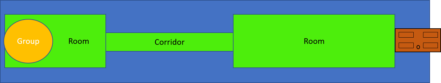
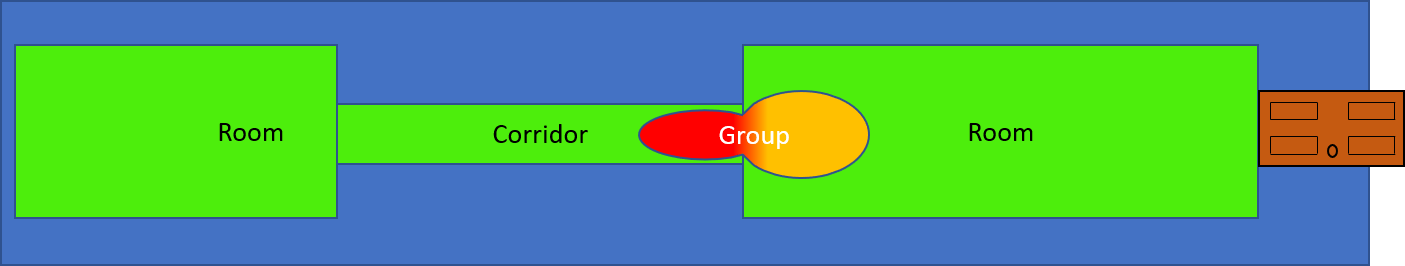
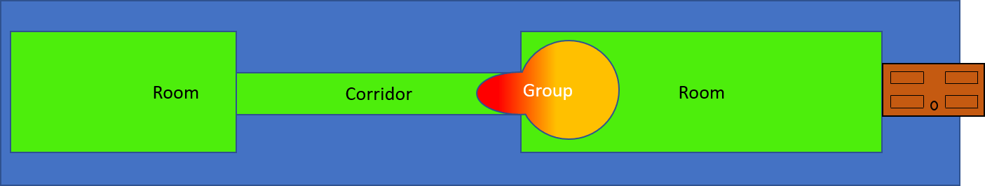
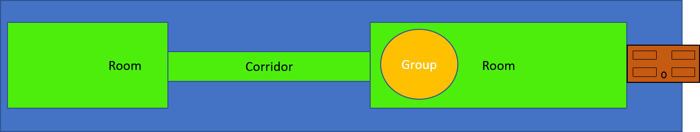
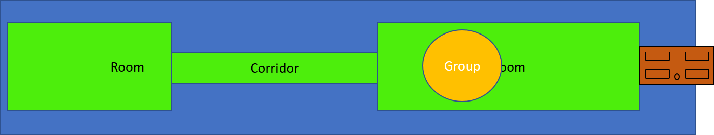
First Order Model:
Furthermore, there are two separate approaches that are used. This website will only go through the first approach (a first order model, FOM), but there are plenty of resources available for readers who want to understand second order approaches. The FOM focuses on finding a single limiting factor in an evacuation. However, this is often a simplification of the situation, and more complex scenarios may not be accurately represented. The process of the FOM is as follows:- Set up parameters, including the maximum flow rates, for each element and transition.
- Find speed and flow rate for first element. $$𝑆 = (1−𝑎)𝑘𝐷$$
-
Ensure flow rate is not above maximum flow rate of all elements and transitions, and specify the limiting factor if it is.
-
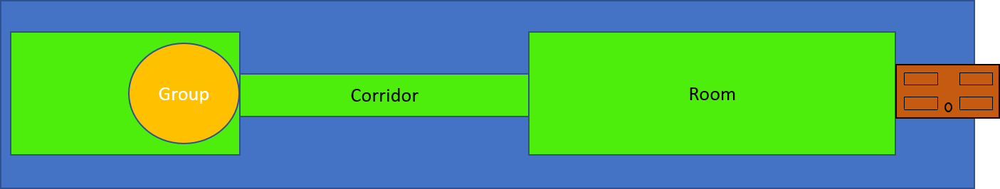
Find the time to traverse the initial element.
$$ T_{element}= \frac{Length_{element}}{Speed_{element}} $$ -
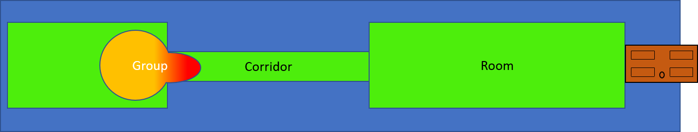
Solve for flow rate and speed across different elements.
$$\begin{align} 𝐹_{out}&=min(𝐹_{in}, 𝐹_{𝑚𝑎𝑥})\\ F_{out}&=(1-aD)kDW_{eff} \\ \\ D&=\frac{\frac{1}{a} \pm \sqrt{\frac{1}{a^2}-4(1)\left(\frac{F_{out}}{akW_{eff}}\right)}}{2} \\ \\ 𝑆 &= (1−𝑎)𝑘𝐷 \end{align}$$-
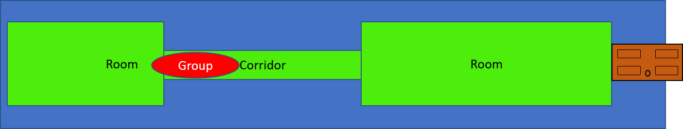
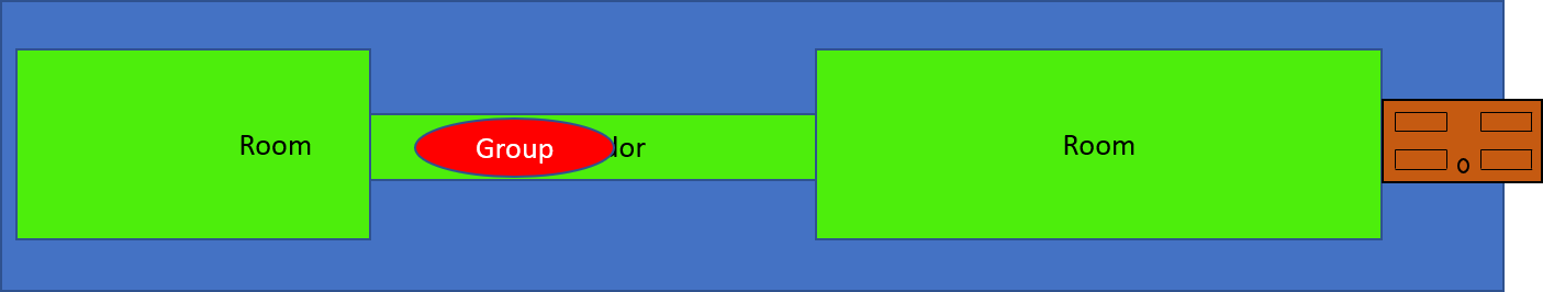
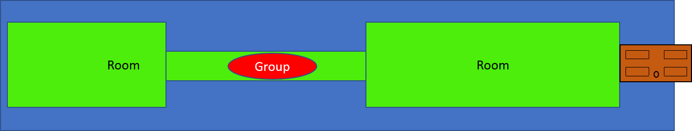
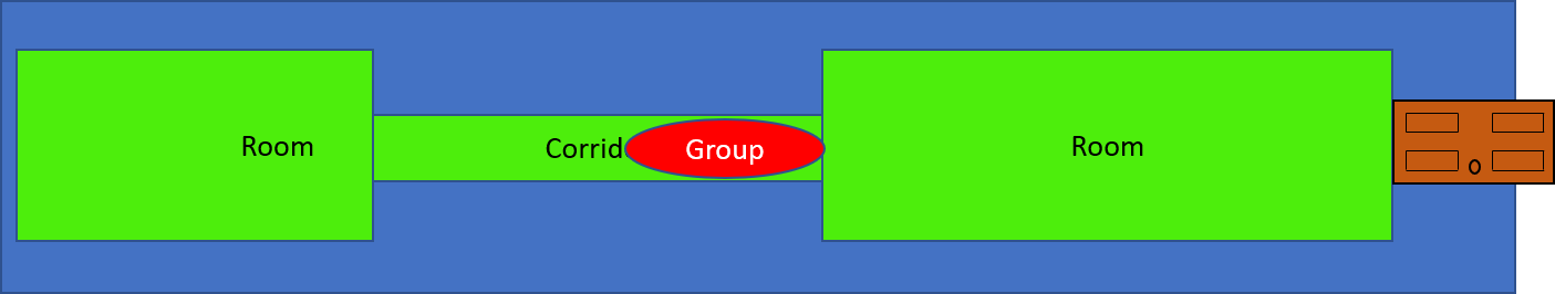
Repeat steps 4 and 5 through all elements, until a queue forms, or until the group has reached their destination.
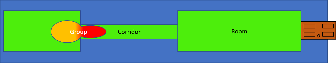
-
If $F_{in} > F_{out}$, then a queue forms. If this happens, repeat steps 4 and 5 for all downstream elements at the reduced flow rate.
-
Repeat steps 4 and 5 through all elements, until a queue forms, or until the group has reached their destination.
- Sum the traversal time for all elements, and the time for any queue to empty.
$$T_{total} = \sum_{i=1}^n T_{element}+T_{queue}$$
Second Order Model (SOM):
The SOM adds a few extra steps to the FOM, allowing for more complex scenarios to be modelled. Specifically, the SOM updates the flow rates at all limiting factors, allowing multiple queues to form as a group moves. $$T_{total} = \sum_{i=1}^n T_{element}+ \sum_{j=1}^m T_{queue}$$ It is worth noting that the SOM approach very quickly becomes intractable to do by hand (especially for a building with multiple groups). The interested reader is referred to the SFPE Handbook of Fire Protection Engineering and this paper for further information.