{{sectionTitleLong[0]}}
A Fourier Series is an expansion of any reasonable (see Dirichlet conditions) periodic function
$ f(x) $ in terms of an infinite sums of sines and cosines,
due to the orthogonality relationships of sines and cosines functions.
Any set of functions that form a complete orthogonal system has a Fourier Series counterpart.
By representing functions in sines and cosines, we have a wide range of tools (differentiation and integration) for analysis that might not be possible in the original function domain.
In this visualisation, we aim to provide a visual approach to understanding how some important periodic functions can be composed using sine and cosine functions.
Try changing the number of terms in the Fourier Series. By increasing this, we can see that the function resembles closer and closer to the square function.
By the end of this suite, you would be able to understand the intuition behind Fourier Series, and to do it yourself for any reasonable periodic function.
By representing functions in sines and cosines, we have a wide range of tools (differentiation and integration) for analysis that might not be possible in the original function domain.
In this visualisation, we aim to provide a visual approach to understanding how some important periodic functions can be composed using sine and cosine functions.
Visualisation Guide
On the right, we can see a square function, and a summation of sines and cosine functions with a finite number of terms that represents the square function.Try changing the number of terms in the Fourier Series. By increasing this, we can see that the function resembles closer and closer to the square function.
By the end of this suite, you would be able to understand the intuition behind Fourier Series, and to do it yourself for any reasonable periodic function.
{{sectionTitleLong[1]}}
Given the vectors $ \vec{V}_{n} $ and $ \vec{V}_{m}, $ we define their
inner product as
$$\vec{V}_{n} \cdot \vec{V}_{m} = \sum_{i}V_{n}^{(i)} V_{m}^{(i)}, $$
where $ V_{n}^{(i)} $ is the $ i^{\text{th}} $
component of the vector
$ \vec{V}_{n}. $ If
$$ \vec{V}_{n} \cdot \vec{V}_{m} = 0 \text{ for } m \neq n, $$
then we say the vectors are orthogonal.
If you move in the direction of any vector $ \vec{a}, $ you do not change the position component in the direction of any vector orthogonal to $ \vec{a}. $ In other words, orthogonal vectors are perpendicular.
If $ \vec{V}_{n} \cdot \vec{V}_{m} = \delta_{nm} $ then the vectors are said to be orthonormal. $$ \delta_{nm} = \left\{\begin{matrix}0 \quad \text{if } m\neq n \\ 1 \quad \text{if } m = n \end{matrix}\right. $$ This mean the vectors are orthogonal and conveniently normalised.
Use the visualisation to see that when the basis vectors are not parallel they span $ \mathbb{R}^{2}, $ using these as basis vectors, we can construct any other vector in $ \mathbb{R}^{2}. $
If you can represent any vector in $ \mathbb{R}^{n} $ using $ n $ vectors, then the basis vectors form a complete set. If the set of these vectors are all orthonormal, then we have a complete orthonormal set.
In the same way as before, we will now demonstrate what it means for functions to be complete. We define the functions $ f_{n},f_{m} $ to exist on the domain $ \left[a,b \right]. $
We define their inner product to be $$ \langle f_{n} , f_{m} \rangle = \int_{a}^{b} f_{n}\left(x \right)f_{m}^{*}\left(x \right)dx $$ , where * denotes the complex conjugate of the function. This is commutative, just like the inner product of two vectors. We say the functions are orthogonal if $ \langle f_{n} , f_{m} \rangle = 0 $ for $ m \neq n. $
We then say the functions are orthonormal if $ \langle f_{n} , f_{m} \rangle = \delta_{nm}, $ where $$ \delta_{nm} = \left\{\begin{matrix}0 \quad \text{if } m\neq n \\ 1 \quad \text{if } m = n \end{matrix}\right. $$ We now claim that you can construct any square integrable function from a complete set of basis functions, in the same way vectors could be constructed from a complete set of basis vectors. A square integrable function $ f $ is a function whose inner product with itself, $ \langle f,f \rangle $ is finite.
{{sectionTitleLong[2]}}
Consider a function $ f(x) $ which is periodic over
the domain $ -L \leq x < L $
where $ L $ is positive. $ f(x) $
can be represented as a sum
of
sines and cosines with varying
frequencies.
These trigonometric functions form orthogonal basis.
The Fourier series of $ f(x) $ is $$ f(x) = \frac{a_0}{2} + \sum_{n=1}^{\infty} \Big[ a_n\cos\Big(\frac{\pi nx}{L}\Big) + b_n\sin\Big(\frac{\pi nx}{L}\Big) \Big] $$ where \begin{align} a_n & = \frac{1}{L}\int_{-L}^{L} f(x) \cos\Big(\frac{\pi nx}{L}\Big) dx, \\ b_n & = \frac{1}{L}\int_{-L}^{L} f(x) \sin\Big(\frac{\pi nx}{L}\Big) dx, \\ \end{align} and $$ n=0,1,2... $$ Note: $ {a_0}/2 $ represents the average value of $ f(x). $
The Fourier series representation of the function $ f(x) $ in exponential (complex) form is $$ f(x) =\sum_{n=-\infty}^{\infty} c_n e^{{in \pi x}/L} \qquad $$ where $$ c_n = \frac{1}{2L}\int_{-L}^{L} f(x) e^{{-in \pi x}/L} dx, $$ Note: The constants in front of the integral(s) of the coefficient for the trigonometric and exponential fourier series are different. Also note the limit of the summations. Follow through the derivation to understand the difference.
We begin by assuming that $ f(x) $ can be represented
as a sum of
exponential terms.
$$ f(x) = \sum_{n=-\infty}^{\infty} c_n e^{{in \pi x}/L} $$
Multiplying by $ e^{{-im \pi x}/L}, $ where $ m=0,1,2,..., $
and integrating both sides gives the following:
$$ \int_{-L}^{L} f(x) e^{{-im \pi x}/L} dx = \sum_{n=-\infty}^{\infty} c_n \int_{-L}^{L} e^{{i(n-m) \pi x}/L} dx. $$
Performing the integral on the R.H.S gives
$$ \int_{-L}^L e^{(i\pi x/L)(n-m)}dx =\left\{ \begin{array}{ll} 2L \qquad \text{(if n=m)} \\
0 \qquad \quad \text{(if n≠m)} \end{array} \right \}=2L\cdot\delta_{nm}. $$
This is the orthonormality of complex exponentials.
Now since the only non-zero value of the sum is when $ n=m, $ $$ \int_{-L}^L f(x) e^{-im\pi x/L}dx = 2L \sum_{n=-\infty}^{+\infty}c_n\delta_{mn} = 2L\cdot c_m, $$ hence $$ c_m=\frac{1}{2L}\int_{-L}^{+L}f(x) e^{-im\pi x/L}dx. $$ Note: As $ m $ is an arbitrary integer, it can be assigned as $ n $ for simplicity.
Given the previously derived equation, we can derive the trigonometric form of the Fourier series. By reorganising the sum, we get $$ f(x)= \underbrace{c_0}_\text{n=0} + \sum_{n=1}^{\infty} \big( \underbrace{c_n e^{in\pi x/L}}_\text{Positive n term} + \underbrace{c_{-n} e^{-in\pi x/L}}_\text{Negative n terms} \big). $$ We can regroup the terms in the summation in the following way:
\begin{align}
f(x)= c_0 + \sum_{n=1}^{\infty} \Big[ & \frac{c_n + c_{-n}}{2} \big(e^{in\pi x/L} +e^{-in\pi x/L} \big) \\
& \frac{c_n - c_{-n}}{2} \big(e^{in\pi x/L} -e^{-in\pi x/L} \big) \Big]
\end{align}
Now define $ a_n = c_n + c_{-n} $ and
$ b_n = i(c_n - c_{-n}) $
and use that these exponentials can we written as
sines and cosines.
Note: $ a_0 = 2c_0 $ and $ b_0=0. $
Hence $$ f(x) = \frac{a_0}{2} + \sum_{n=1}^{\infty} \Big[ a_n\cos\Big(\frac{\pi nx}{L}\Big) + b_n\sin\Big(\frac{\pi nx}{L}\Big) \Big] $$ $ a_n $ can be derived by using the expression from $ c_n $ \begin{align} a_n = c_n + c_{-n} = & \frac{1}{2L}\int_{-L}^{+L}f(x) e^{-in\pi x/L}dx \\ + & \frac{1}{2L} \int_{-L}^{+L}f(x) e^{in\pi x/L}dx \end{align} Factorise and spot the exponential form of $ \cos. $ \begin{align} & =\frac{1}{L}\int_{-L}^{+L}f(x) \Big[\frac{e^{in\pi x/L} +e^{-in\pi x/L}}{2}\Big]dx \\ & =\frac{1}{L}\int_{-L}^{L} f(x) \cos\Big(\frac{\pi nx}{L}\Big) dx \end{align} Similarly for $ b_n, $ $$ b_n =\frac{1}{L}\int_{-L}^{L} f(x) \sin\Big(\frac{\pi nx}{L}\Big) dx. $$
Now since the only non-zero value of the sum is when $ n=m, $ $$ \int_{-L}^L f(x) e^{-im\pi x/L}dx = 2L \sum_{n=-\infty}^{+\infty}c_n\delta_{mn} = 2L\cdot c_m, $$ hence $$ c_m=\frac{1}{2L}\int_{-L}^{+L}f(x) e^{-im\pi x/L}dx. $$ Note: As $ m $ is an arbitrary integer, it can be assigned as $ n $ for simplicity.
Given the previously derived equation, we can derive the trigonometric form of the Fourier series. By reorganising the sum, we get $$ f(x)= \underbrace{c_0}_\text{n=0} + \sum_{n=1}^{\infty} \big( \underbrace{c_n e^{in\pi x/L}}_\text{Positive n term} + \underbrace{c_{-n} e^{-in\pi x/L}}_\text{Negative n terms} \big). $$ We can regroup the terms in the summation in the following way:
\begin{align}
= \frac{1}{2} \Big[ 2c_n e^{in\pi x/L} + 2c_{-n} e^{-in\pi x/L} & \\
+ \underbrace{c_{-n} e^{in\pi x/L} - c_{-n} e^{in\pi x/L}}_\text{ =0} & \\
+ \underbrace{c_{n} e^{-in\pi x/L} -c_{n} e^{-in\pi x/L}}_\text{ =0} & \Big] \\
\end{align}
\begin{align} = \frac{1}{2} \Big[ c_n e^{in\pi x/L} +c_{-n} e^{in\pi x/L} & \\ + c_n e^{-in\pi x/L} + c_{-n} e^{-in\pi x/L} & \\ + c_n e^{in\pi x/L} - c_{-n} e^{in\pi x/L} & \\ - c_n e^{-in\pi x/L} + c_{-n} e^{-in\pi x/L} & \Big] \\ \end{align}
\begin{align} = \frac{1}{2} \Big[ c_n e^{in\pi x/L} +c_{-n} e^{in\pi x/L} & \\ + c_n e^{-in\pi x/L} + c_{-n} e^{-in\pi x/L} & \\ + c_n e^{in\pi x/L} - c_{-n} e^{in\pi x/L} & \\ - c_n e^{-in\pi x/L} + c_{-n} e^{-in\pi x/L} & \Big] \\ \end{align}
Note: $ a_0 = 2c_0 $ and $ b_0=0. $
Hence $$ f(x) = \frac{a_0}{2} + \sum_{n=1}^{\infty} \Big[ a_n\cos\Big(\frac{\pi nx}{L}\Big) + b_n\sin\Big(\frac{\pi nx}{L}\Big) \Big] $$ $ a_n $ can be derived by using the expression from $ c_n $ \begin{align} a_n = c_n + c_{-n} = & \frac{1}{2L}\int_{-L}^{+L}f(x) e^{-in\pi x/L}dx \\ + & \frac{1}{2L} \int_{-L}^{+L}f(x) e^{in\pi x/L}dx \end{align} Factorise and spot the exponential form of $ \cos. $ \begin{align} & =\frac{1}{L}\int_{-L}^{+L}f(x) \Big[\frac{e^{in\pi x/L} +e^{-in\pi x/L}}{2}\Big]dx \\ & =\frac{1}{L}\int_{-L}^{L} f(x) \cos\Big(\frac{\pi nx}{L}\Big) dx \end{align} Similarly for $ b_n, $ $$ b_n =\frac{1}{L}\int_{-L}^{L} f(x) \sin\Big(\frac{\pi nx}{L}\Big) dx. $$
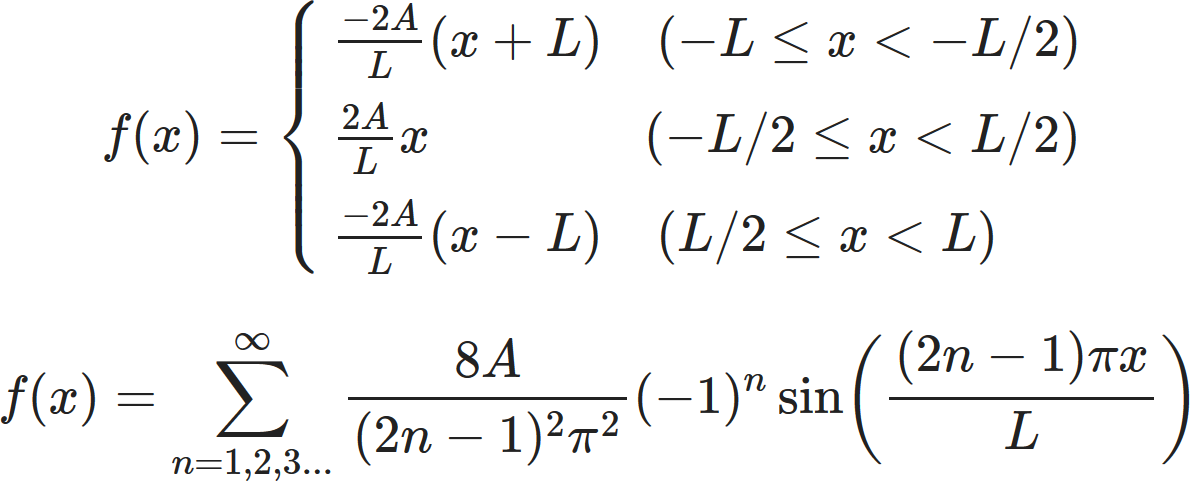
The triangular function is defined by the following:
$$ f(x)=\left\{
\begin{array}{ll}
\frac{-2A}{L} (x+L) \quad (-L \leq x < -L/2) \\
\frac{2A}{L} x \qquad \qquad (-L/2\leq x < L/2) \\
\frac{-2A}{L} (x-L) \quad (L/2\leq x < L)
\end{array}
\right. $$
First notice that $ f(x) $ is odd about $ x=0, $ hence $ a_n=0 $
for all $ n. $ Also, since the $ b_n $ integrand is even about
$ x=0, $
$$ b_n=\frac{2}{L}\int_0^L f(x) \sin \left(\frac{n \pi x}{L}\right)dx. $$
Notice that for even $ n, $ $ b_n $ is odd about
$ x=L/2. $
Hence,
$$ b_n=\frac{2}{L}\int_0^{L} f(x) \sin \left(\frac{n\pi x}{L} \right) dx = 0 \quad \text{for even n}. $$
The integral from $ 0 $ to $ L/2 $ is equal in magnitude but
opposite in sign to the integral from $ L/2 $ to
$ L, $ for
even $ n. $
For odd $ n, $ the function is even around $ L/2, $ so we only have to integrate from $ 0 $ to $ L/2 $ then multiply by $ 2. $ This has made our job much easier. $$ b_n=2\frac{2}{L}\int_0^{L/2} f(x) \sin \left(\frac{n\pi x}{L} \right) dx \quad \text{for odd n} $$ Play around with the visualisation to the right to convince yourself this is true.
For odd $ n, $ the function is even around $ L/2, $ so we only have to integrate from $ 0 $ to $ L/2 $ then multiply by $ 2. $ This has made our job much easier. $$ b_n=2\frac{2}{L}\int_0^{L/2} f(x) \sin \left(\frac{n\pi x}{L} \right) dx \quad \text{for odd n} $$ Play around with the visualisation to the right to convince yourself this is true.
$$ \text{For 0 < x < L/2:} \quad f(x)=\frac{2Ax}{L} $$
Remembering that for even $ n, $ $ b_n=0, $ therefore only
consider odd $ n. $
$$ b_n = \frac{4}{L} \frac{2A}{L}\int_0^{L/2} x \sin \left(\frac{n\pi x}{L} \right) dx $$
This integral can be performed by parts.
$$ b_n=\frac{8A}{L^2} \frac{L^2}{(n\pi)^2} \sin \left(\frac{n\pi x}{L} \right) \biggr |_0^{L/2} $$
Note for odd $ n $:
$$ \sin \left(\frac{n\pi}{2} \right)=(-1)^{\frac{n-1}{2}} $$
Therefore,
$$ b_n=\frac{8A}{n^2\pi^2}(-1)^{\frac{n-1}{2}} $$
and,
$$ f(x)=\sum_{n=1,3,5...}^\infty \frac{8A}{n^2\pi^2} (-1)^{\frac{n-1}{2}} \sin \left(\frac{n\pi x}{L} \right) $$
Finally, using the fact that odd number can be written as $ 2n +1 $ for any integer
$ n, $ we have
$$ f(x)=\sum_{n=1,2,3...}^\infty \frac{8A}{(2n-1)^2\pi^2}(-1)^n \sin \left(\frac{(2n-1)\pi x}{L} \right) $$
$$ u=x \qquad dv= \sin \left(\frac{n\pi x}{L} \right)dx $$
$$ du=dx \qquad v=\frac{-L}{n\pi} \cos \left(\frac{n\pi x}{L} \right) $$
\begin{align}
b_n=\frac{8A}{L^2} \Bigg[ \Big[ \frac{-xL}{n\pi} & \cos \Big(\frac{n\pi x}{L}\Big) \Big] \Bigr|_0^{L/2} \\
-\int_0^{L/2}\frac{-L}{n\pi} & \cos \Big(\frac{n\pi x}{L} \Big)dx \Bigg]
\end{align}
For odd n,
$$ \cos \left(\frac{n\pi}{2} \right)=0 $$
Therefore,
$$ b_n=\frac{8A}{L^2} \Bigg[0+ \int_0^{L/2}\frac{L}{n\pi} \cos \left(\frac{n\pi x}{L}
\right)dx \Bigg] $$
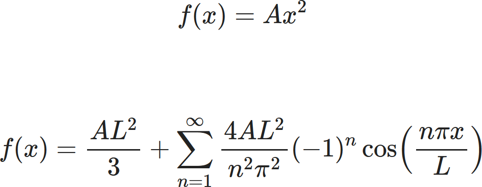
The parabolic function is defined as:
$$ f(x)=Ax^2 \quad \text{for:} -L\leq x< L $$
and is forced to be periodic. $ A $ is a constant.
Therefore, the coefficients $ a_n $ and $ b_n $
are given by
$$ b_n = \frac{1}{L}\int_{-L}^{+L} Ax^2 \sin \left(\frac{n \pi x}{L} \right)dx $$
$$ a_n= \frac{1}{L}\int_{-L}^{+L} Ax^2 \cos \left(\frac{n \pi x}{L} \right)dx $$
The $ b_n $ integral is odd about $ x=0, $ hence
$ b_n=0 $ for all $ n. $ $ f(x) $ is
even about
$ x=0. $ Thus,
$$ a_n=\frac{2}{L}\int_{0}^{+L} Ax^2 \cos \left(\frac{n \pi x}{L} \right)dx. $$
For $ n=0 $:
$$ a_0 = \frac{2}{L} \int _{0}^{+L} Ax^2 dx = \frac{2AL^2}{3} $$
For $ n\neq 0 $:
$$ a_n = \frac{2A}{L}\int_0^L x^2 \cos \left(\frac{n\pi x}{L} \right)dx $$
This equation can now be solved using integration by parts.
$$ a_n = -\frac{4A}{n\pi}\int_{0}^{L} x \sin \left(\frac{n \pi x}{L} \right)dx $$
$$ a_n = \frac{4A}{n\pi} \Bigg[\frac{xL}{n\pi} \cos \left(\frac{n\pi x}{L} \right) \Bigg] \biggr |_0^L $$
$$ = \frac{4AL^2}{n^2\pi^2}(-1)^n $$
Therefore, the fourier series can be written as
$$ f(x) = \frac{AL^2}{3} + \sum_{n=1}^\infty \frac{4AL^2}{n^2\pi^2} (-1)^n \cos \left(\frac{n\pi x}{L} \right) $$
$$ du = 2x\cdot dx \qquad v=\frac{L}{n\pi} \sin \left(\frac{n\pi x}{L} \right) $$
$$ u=x^2 \qquad dv= \cos \left(\frac{n \pi x}{L} \right)dx $$
\begin{align}
a_n = \frac{2A}{L} \Bigg[ \Big[\frac{Lx^2}{n\pi} & \sin \left(\frac{n\pi x}{L} \right) \Big] \biggr |_0^L \\
-\int_0^L\frac{2xL}{n\pi} & \sin \left(\frac{n \pi x}{L} \right)dx \Bigg]
\end{align}
$$ = \frac{2A}{L} \Bigg[0 -\int_0^L\frac{2xL}{n\pi} \sin\left(\frac{n \pi x}{L}\right)dx \Bigg] $$
$$ u = x \qquad dv = \sin \left(\frac{n\pi x}{L} \right) dx $$
$$ du = dx \qquad v = -\frac{L}{n\pi} \cos \left(\frac{n\pi x}{L} \right) $$
\begin{align}
a_n = \frac{-4A}{n\pi} \Bigg[\Big[-\frac{xL}{n\pi} & \cos \left(\frac{n\pi x}{L} \right)\Big] \biggr |_0^L \\
- \int_0^L\frac{-L}{n\pi} & \cos \left(\frac{n\pi x}{L} \right)dx \Bigg]
\end{align}
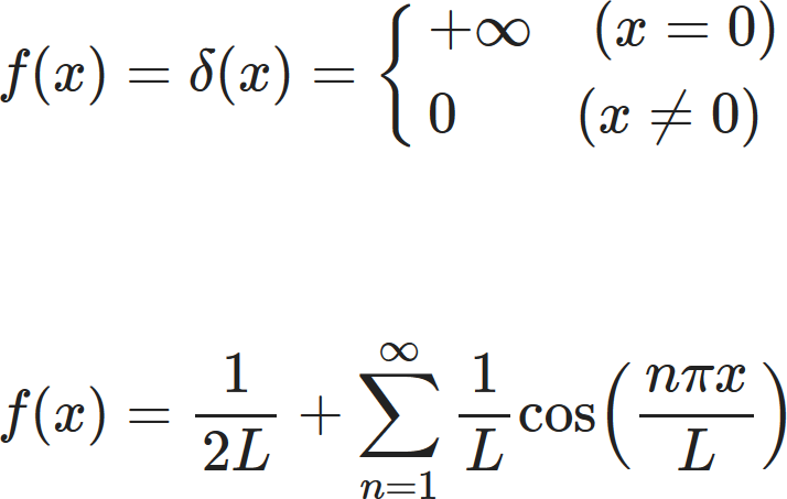
The Dirac-delta function can be thought of as a infinite spike at $ x=0. $
$$
f(x) = \delta(x)=\left\{
\begin{array}{ll}
+\infty \quad (x=0) \\
0 \qquad (x \neq 0)
\end{array}
\right.
$$
$$ a_n=\frac{1}{L}\int_{-L}^{+L} \delta (x) \cos \left(\frac{n\pi x}{L} \right)dx $$
$$ b_n=\frac{1}{L}\int_{-L}^{+L}\delta(x) \sin \left(\frac{n\pi x}{L} \right)dx $$
$ \delta(x) $ is an even function. Hence $ b_n=0 $ and
$$ a_n=\frac{1}{L} $$
Therefore, the fourier series for positive $ L $ can
be written as
$$ f(x)=\frac{1}{2L}+\sum_{n=1}^\infty \frac{1}{L} \cos \left(\frac{n\pi x}{L} \right). $$
By considering the shifting property of the Dirac-Delta function,
$$ \int_{\alpha-\epsilon}^{\alpha+\epsilon} g(x) \delta(x-\alpha)dx=g(\alpha) $$
For us, $ \alpha=0, $ $ \epsilon=L, $ and $ g(x)= \sin \left(n \pi x/L \right). $
Therefore, $$ a_n=\frac{1}{L}\cos \left(\frac{n\pi \times 0}{L} \right)=\frac{1}{L} $$ $$ b_n=\frac{1}{L}\sin \left(\frac{n\pi \times 0}{L} \right)=0 $$
Therefore, $$ a_n=\frac{1}{L}\cos \left(\frac{n\pi \times 0}{L} \right)=\frac{1}{L} $$ $$ b_n=\frac{1}{L}\sin \left(\frac{n\pi \times 0}{L} \right)=0 $$
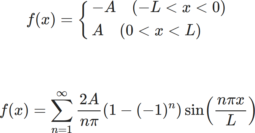
The square wave is defined as the following:
$$
f(x)=\left\{
\begin{array}{ll}
-A \quad (-L \leq x < 0) \\
A \quad (0\leq x < L)
\end{array}
\right.
$$
The $ a_{n} $ terms can be found be noting that $ f(x) $ is
odd,
so $ a_n $ is $ 0 $ for all $ n. $
To find the $ b_n $ terms, the integration can be split into two parts: $ -L\leq x <0 $ and $ 0\leq x < L. $
This gives the following integration: \begin{align} b_n & =\frac{1}{L}\int_{-L}^0 -A \sin \left(\frac{n\pi x}{L} \right)dx \\ & + \frac{1}{L}\int_0^L A \sin \left(\frac{n \pi x}{L} \right)dx \end{align} which can be evaluated to: $$ b_n=\frac{-2A}{L}\frac{L}{n\pi} \cos \left(\frac{n\pi x}{L} \right)\biggr |_0^L =\frac{2A}{n\pi}\left[1-\cos\left(n\pi \right) \right] $$ Note that $$ \cos \left(n \pi\right)=(-1)^n $$ Hence $$ b_n=\frac{2A}{n\pi}(1-(-1)^n) $$ Therefore the final fourier series is: $$ f(x)=\sum_{n=1}^{\infty} \frac{2A}{n\pi} (1-(-1)^n)\sin \left(\frac{n\pi x}{L}\right). $$
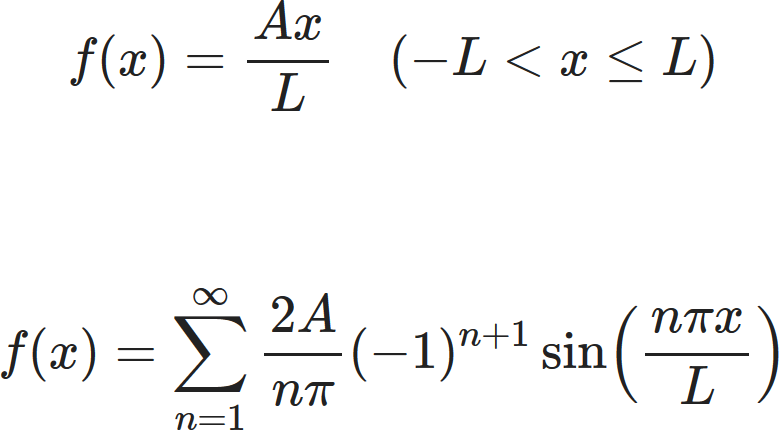
The Sawtooth wave is defined as the following:
$$ f(x)=\frac{Ax}{L} \quad (-L \leq x < L). $$
$ f(x) $ is odd, so $ a_n= 0 $
for all $ n. $
The $ b_n $ terms are given by the following integration: \begin{align} b_n & =\frac{1}{L}\int_{-L}^{L} \frac{Ax}{L}\sin \left(\frac{n\pi x}{L} \right)dx \\ & =\frac{2A}{L^{2}}\int_{0}^{L} x \sin \left(\frac{n\pi x}{L} \right)dx. \end{align} Using Integration by parts it can be shown that:
$$ b_n=\frac{2A}{n\pi}(-1)^{n+1}. $$
Therefore the final fourier series is:
$$ f(x)=\sum_{n=1}^\infty \frac{2A}{n\pi}(-1)^{n+1} \sin \left(\frac{n\pi x}{L} \right). $$
The $ b_n $ terms are given by the following integration: \begin{align} b_n & =\frac{1}{L}\int_{-L}^{L} \frac{Ax}{L}\sin \left(\frac{n\pi x}{L} \right)dx \\ & =\frac{2A}{L^{2}}\int_{0}^{L} x \sin \left(\frac{n\pi x}{L} \right)dx. \end{align} Using Integration by parts it can be shown that:
$$ u=x \quad dv=\sin \left(\frac{n\pi x}{L} \right)dx $$
$$ du=dx \quad v=\frac{-L}{n\pi}\cos \left(\frac{n\pi x}{L} \right) $$
\begin{align}
b_n=\frac{2A}{L^{2}} \Bigg[ \frac{-Lx}{n\pi} & \cos \left(\frac{n\pi x}{L} \right)\biggr |_0^L \\
-\int_0^L\frac{-L}{n\pi} & \cos \left(\frac{n\pi x}{L} \right)dx \Bigg]
\end{align}
Note that the second integrand is zero as it is of cosine over a full
period.
$$ b_n=-\frac{2A}{n\pi} \cos \left(n\pi \right)=-\frac{2A}{n\pi}(-1)^n $$
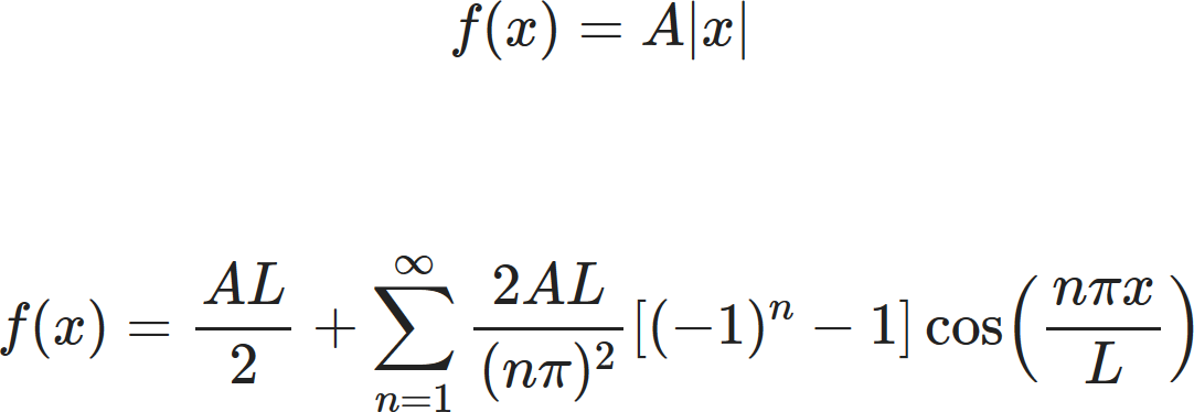
The $ |x| $ function is defined as the following:
$$ f(x)=A|x| \quad (-L \leq x < L). $$
$$ a_n = \frac{1}{L}\int_{-L}^{+L} A|x| \cos \left(\frac{n \pi x}{L} \right)dx $$
$$ b_n = \frac{1}{L}\int_{-L}^{+L} A|x| \sin \left( \frac{n\pi x}{L}\right) dx $$
$ f(x) $ is even about $ x=0. $
Hence $ b_n=0. $
The $ a_n $ integral is even about $ x=0. $ Hence,
$$ a_n = \frac{2}{L}\int_{0}^{+L} Ax \cos \left(\frac{n \pi x}{L}\right)dx. $$
For $ n=0 $
$$ a_0 = \frac{2A}{L}\int_0^L x dx = \frac{2A}{L}\frac{x^2}{2} \biggr |_0^L = AL. $$
For $ n \neq 0 $:
$$ a_n = \frac{2A}{L}\int_{0}^{+L} x \cos \left(\frac{n \pi x}{L} \right)dx. $$
By integrating by parts,
$$ a_n = \frac{2A}{L}\frac{L^2}{(n\pi)^2} \cos \left( \frac{n\pi x}{L} \right)\biggr |_0^L . $$
Hence,
$$ a_n = \frac{2A}{L}\frac{L^2}{(n\pi)^2} \left[(-1)^n-1 \right] = \frac{2AL}{(n\pi)^2}\left[(-1)^n-1 \right]. $$
Therefore the final fourier series is:
$$ f(x)=\frac{AL}{2}+ \sum_{n=1}^\infty \frac{2AL}{(n\pi)^2} \left[(-1)^n-1 \right] \cos \left(\frac{n\pi
x}{L} \right). $$
$$ u=x \qquad dv= \cos\left(\frac{n\pi x}{L}\right)dx $$
$$ du=dx \qquad v=\frac{L}{n\pi} \sin \left(\frac{n\pi x}{L} \right) $$
\begin{align}
a_n = \frac{2A}{L} \Bigg[ \Big[\frac{Lx}{n\pi} & \sin \left( \frac{n \pi x}{L} \right) \Big] \Biggr|_0^L \\
-\int_0^{+L} \frac{L}{n\pi} & \sin \left(\frac{n \pi x}{L} \right)dx \Bigg]
\end{align}
$$ a_n = \frac{2A}{L} \Bigg[ 0 -\int_0^{+L}\frac{L}{n\pi} \sin \left(\frac{n\pi x}{L} \right)dx \Bigg] $$
{{sectionTitleLong[3]}}
The 0th term of the series, $ \frac{a_0}{2}, $ is the
constant term before the sum.
This is labelled as the 0th term so that the series may start indexing its terms from $ n=1. $ $$ f(x)=\frac{a_0}{2}+\sum_{n=1}^{\infty}a_n \cos\left(\frac{n\pi x}{L}\right)+b_n \sin\left(\frac{n \pi x}{L}\right) $$ If the function is not periodic, then we may cut the function, forcing it to be periodic over some $ -L < x < L. $ This means that we can prescribe a Fourier series that is now valid for the function over the selected range. If we take the limit as $ L \rightarrow \infty, $ then a Fourier transform need be used. This is a different problem entirely!
This is labelled as the 0th term so that the series may start indexing its terms from $ n=1. $ $$ f(x)=\frac{a_0}{2}+\sum_{n=1}^{\infty}a_n \cos\left(\frac{n\pi x}{L}\right)+b_n \sin\left(\frac{n \pi x}{L}\right) $$ If the function is not periodic, then we may cut the function, forcing it to be periodic over some $ -L < x < L. $ This means that we can prescribe a Fourier series that is now valid for the function over the selected range. If we take the limit as $ L \rightarrow \infty, $ then a Fourier transform need be used. This is a different problem entirely!
{{sectionTitleLong[4]}}
Decomposition of a function into odd and even parts
Representing a function in terms of a trigonometric Fourier series is analogous to representing a vector in terms of basis vectors. Here sines and cosines are our basis functions, we have a method for finding the projection of the function in the direction of each basis function ($ a_{n} $ and $ b_{n} $ are the "projections" of $ f(x) $ onto $ \sin\left(\frac{n\pi x}{L} \right) $ and $ \cos\left(\frac{n \pi x}{L} \right) $ respectively).This visualisation shows how the first ten terms are introduced to the series, notice that usually as the number of terms included in the series increases, new terms become less significant (their amplitude decreases).
Power Spectrum
The power spectrum form is a different representation of a continuous signal.One can think of a signal as a sound wave that is a superposition of different frequencies $ \omega_n, $ each with amplitude $ \alpha_n, $ and relative phases $ \theta_n. $ Any signal of period $ 2L $ can be decomposed in terms of the amplitude and relative phase of its discrete frequency modes. Its two parameters $ \alpha_n $ and $ \theta_n, $ enable us to measure the amount of each frequency $ \omega_n=\frac{n\pi}{L} $contained in the signal, and the relative phase difference between the $ n^{th} $ frequency and a cosine wave centered at $ x=0. $ This is simply a different way to represent a signal rather than decomposing it into its even and odd parts. $$ f(x) = \frac{a_0}{2} + \sum_{n=1}^{\infty}\alpha_n \cos\bigg(\frac{n\pi x}{L} - \theta_n\bigg) $$ $$ \alpha_n = \sqrt{a^2_n + b^2_n} $$ $$ \theta_n = \tan^{-1} \bigg(\frac{b_n}{a_n}\bigg) $$ For some even functions, when the period transitions from 0 to negative, the value of $ \theta_n $ change from $ 0 $ to $ \pi $ or vice versa. Why do you think this happens?
This happens because the value of $ a_n $ changes sign
($ b_n $ is 0) causing the value of
$ \theta_n $ to change. For $ b_n = 0, $
$ \tan^{-1}(\frac{b_n}{a_n}) $
can be both
0 or $ \pi $ depending on whether $ a_n $ is positive or
negative. Not all even functions exhibit this.
The parabola for example, has its $ a_n $ proportional to
$ L^2, $ so its sign does not change when $ L $ changes
sign.
Orthogonal functions
Two functions $ f $ and $ g $ are said to be orthogonal if their inner product $ \langle f,g\rangle $ is 0. Just like basis vectors in a finite vector space, a set of orthogonal functions can form an infinite basis in a function space and a linear sum of these basis functions can describe any function in that function space.For functions that are periodic over $ -L < x \leq L $ with a period of $ 2L, $ the fourier components $ \rightarrow $ $ \sin(\frac{\pi x}{L}), \cos(\frac{\pi x}{L}), \sin(\frac{2\pi x}{L}), \cos(\frac{2\pi x}{L})... $ and so on form a complete orthogonal set that can be used to describe these functions. This means that increasing the amplitude of one of the components does not affect the other components, so changing the amount of any frequency contained in a signal leaves all the other frequencies unaffected.
{{sectionTitleLong[5]}}
Description
Finally, you can see the components of the series, the power spectrum and the resultant Fourier series displayed all at once. You can select one of the example functions from the previous sections, or input your own custom function, and see how all the elements work together to build a Fourier series.How To Use Custom Functions
To specify a custom function, select custom from the drop down menu and input your desired function into the input for $ f(x). $The period slider forces the function you have specified to be periodic over $ -L < x \leq L. $ For example if $ f(x) = \sin(x) $ with $ L = 1, $ this is the sine function but cut at $ x = \pm 1 $ and forced to be periodic over just this range (not the full $ 2\pi $ period).
The following functions can be used:
- Trigonometric functions (e.g. sin(), cos())
- Trigonometric inverses (e.g. arcsin(), arccos())
- Hyperbolic functions (e.g. sinh(), cosh())
- Hyperbolic inverses (e.g. arsinh(), arcosh())
- Exponentials and logs (e.g. exp(), log())
Syntax
Entering $ 5x $ does not work: instead you should write 5*x.Write exponents as a^(exponent), so $ x^2 $ is written as x^2.
Functions should be real and fully defined over the domain, for example $ log(x) $ is imaginary for values less than zero, so does not work.
$ log(x+1) $ does not work either (with a period of 1), since log is undefined at zero, however $ log(1+x^2) $ does work for all periods, since it is defined over the whole domain and is real.
{{sectionTitleLong[6]}}
In a Fourier Series, if the range over which the function is periodic, $ L $
goes to infinity, this function is no longer periodic.
To treat such a function, we would use Fourier Transform.
At its core, the Fourier Transform converts the function from one domain to another.
For example, by performing a Fourier Transform of a wave packet in the time domain, we can transform the wave packet into the frequency domain. This can make analysis (such as differentiation) much easier than performing it in the original domain.
One major application of Fourier Transform is in sound signal editing. Sound data is picked up by a microphone which records the pressure variation of air against time. When a Fourier Transform is performed, the relative intensities of the constituent frequencies that make up the signal is broken down, making it easier for sound correction and timbre analysis.
The Fourier Transform graph gives the relative "intensity" of the respective frequencies that make up the top-hat graph.
At its core, the Fourier Transform converts the function from one domain to another.
For example, by performing a Fourier Transform of a wave packet in the time domain, we can transform the wave packet into the frequency domain. This can make analysis (such as differentiation) much easier than performing it in the original domain.
One major application of Fourier Transform is in sound signal editing. Sound data is picked up by a microphone which records the pressure variation of air against time. When a Fourier Transform is performed, the relative intensities of the constituent frequencies that make up the signal is broken down, making it easier for sound correction and timbre analysis.
Visualisation Guide
On the left, we see a top-hat function that we intend to perform a Fourier Transform on. The graph on the right shows the Fourier Transform of the top hat function. We have represented the top hat graph in the frequency space.The Fourier Transform graph gives the relative "intensity" of the respective frequencies that make up the top-hat graph.